Tutorial 3 - Plot extracted spectra

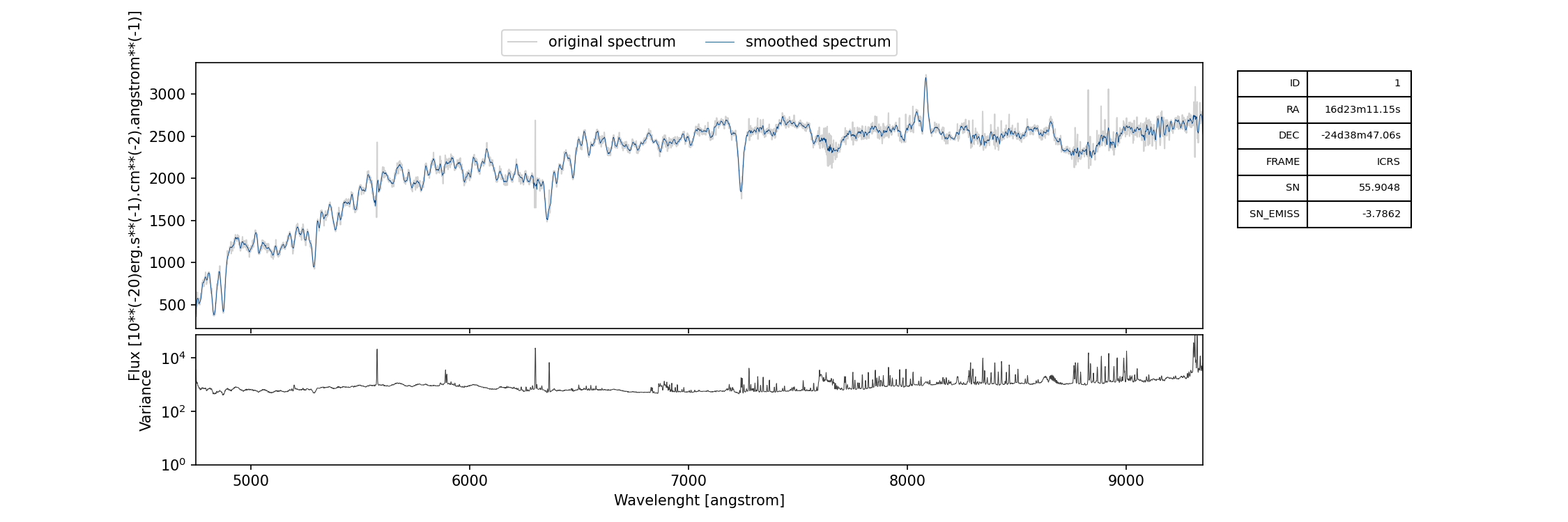
Using the same data and spectra extracted in the first tutorial, we can generate the plots of the extracted spectra using the command spec_1.png:

specex-plot --outdir extraced_spectra_plots extracted_spectra/spec_*.fits

the parameter --outdir is used to set the folder where to save the plots. This is, for example, the plot of spec_1.fits

The plot of a spectrum generated using *specex-plot*.

We can also specify the smoothing to apply to the spectrum before plotting using the parameter --smoothing that accepts as input an integer greater or equal to 0, where 0 means no smoothing. We can also specify an image from which to extract a cutout of the source using the parameter --cutout and the size of the cutout itself can be set using the parameter --cutout-size. For example, if we want to include a cutout of 5” from the whitelight image and plot the spectra with a smoothing window of size of 3, we can use the command

specex-plot --smoothing 3 --cutout ADP.2023-09-01T12_56_41.595_data.fits --cutout-size 5arcsec --outdir extraced_spectra_plots_smooth_3 extracted_spectra/spec_*.fits

that generates plots which will be like the following one

The plot of a spectrum generated using *specex-plot* with a cutout from the whitelight image.

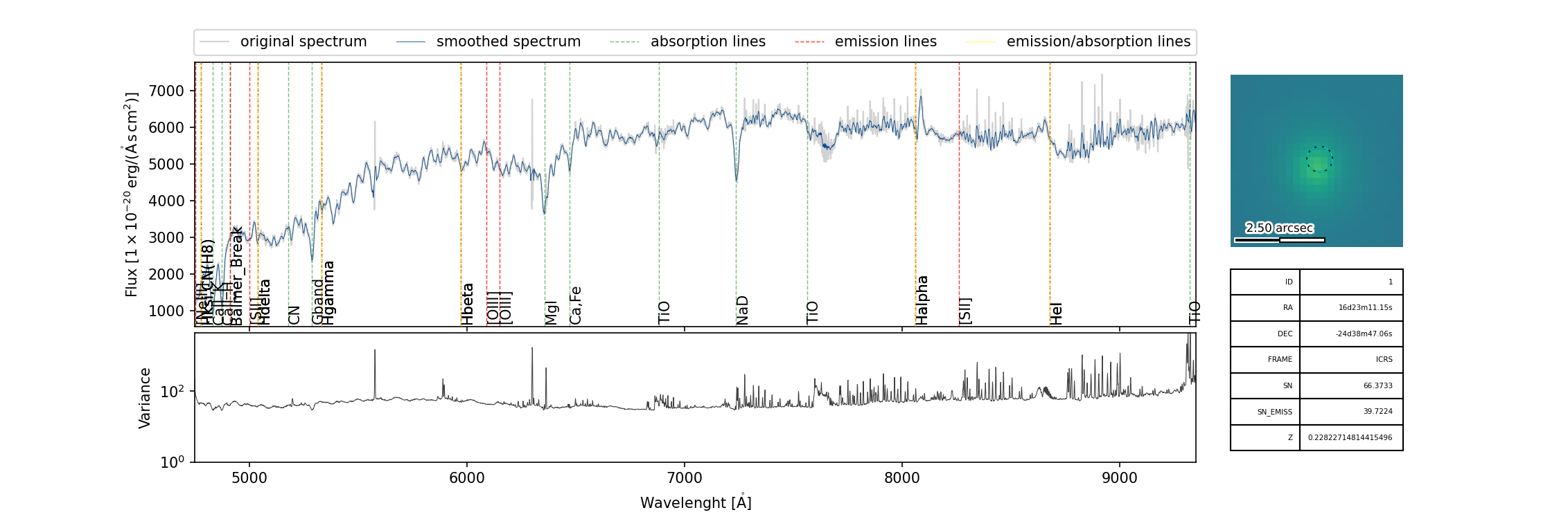
If a redshift catalog is available, it can be used to overlay on the spectrum plot the most common absorption/emission lines and can be set using --zcat. If this catalog has not been generate by rrspecex, the name of the columns containing the IDs of the objects and their redshift can be specified using the parameters --key-id and --key-z, for example

specex-plot --zcat zbest_wsum.fits --key-id SPECID --key-z Z --smoothing 3 --cutout ADP.2023-09-01T12_56_41.595_data.fits --cutout-size 5arcsec --outdir spectra_plots_wsum_zcat extracted_spectra_wsum/spec_*.fits

will produce plots like this one